Prevent look-ahead bias
I applied a one-day prior-close signal lag before assigning each regime.
Statistical Analytics · Data Validation
A regime analysis that tests bias, threshold sensitivity, uncertainty, and cross-system agreement.
My approach
I applied a one-day prior-close signal lag before assigning each regime.
I tested six VIX and yield threshold combinations and compared asset metrics by regime.
I used 5,000 moving-block bootstrap resamples and reconciled outputs across Python and PostgreSQL.
Analytical trust
The validation path challenges the finding before it is presented.
The initial result identifies a regime relationship.
Six threshold combinations test the classification.
The stability test supports the descriptive finding.
Decision evidence
Point estimates are shown with method controls and uncertainty, not presented as forecasts.
Why this visual exists. Return, risk, drawdown, Sharpe ratio, and correlation are read together across four lagged regimes.
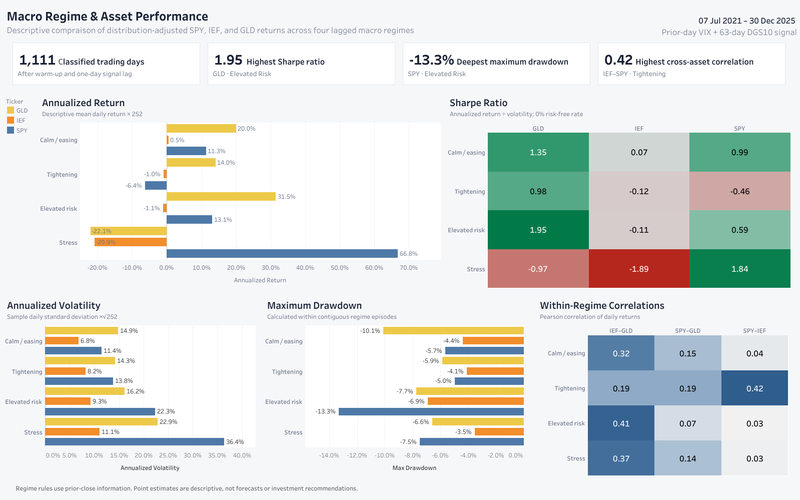
GLD has the highest Sharpe ratio at 1.95 in Elevated risk. SPY has the deepest maximum drawdown at −13.3% in the same regime.
No single metric defines performance. Return must be read with volatility, drawdown, and cross-asset behaviour.
Use the dashboard to select claims for robustness checks, not to issue an investment recommendation.
Why this visual exists. A common return view makes direction and magnitude easy to compare before testing uncertainty.
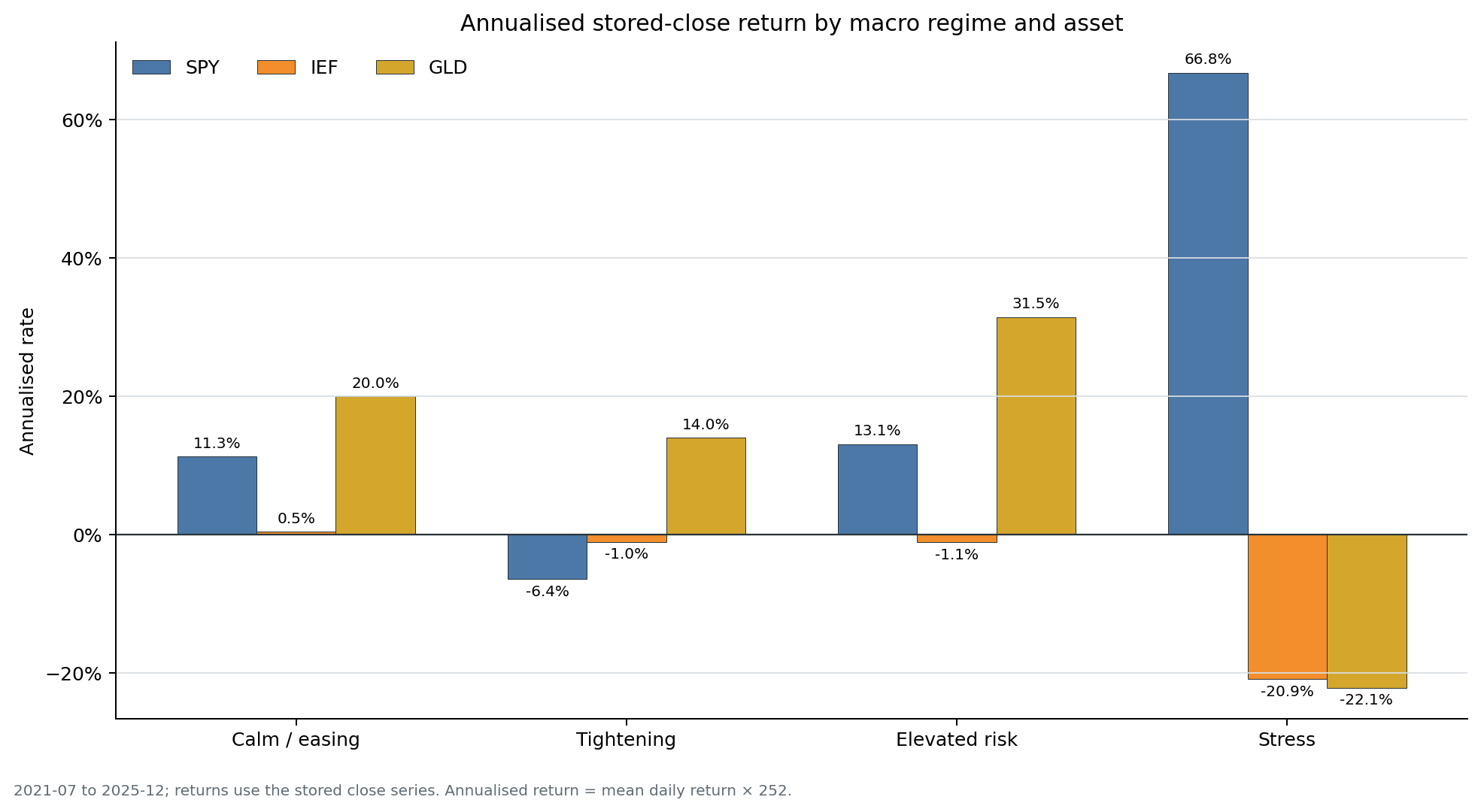
SPY is 66.8% annualised in Stress, while IEF and GLD are −20.9% and −22.1%. GLD is 31.5% in Elevated risk.
These are descriptive annualised sample means. The Stress estimate can be unstable because regime samples are limited.
Do not use magnitude alone. Check sensitivity and sampling uncertainty before retaining the claim.
Why this visual exists. Moving-block bootstrap intervals preserve short time dependence and expose imprecise regime estimates.
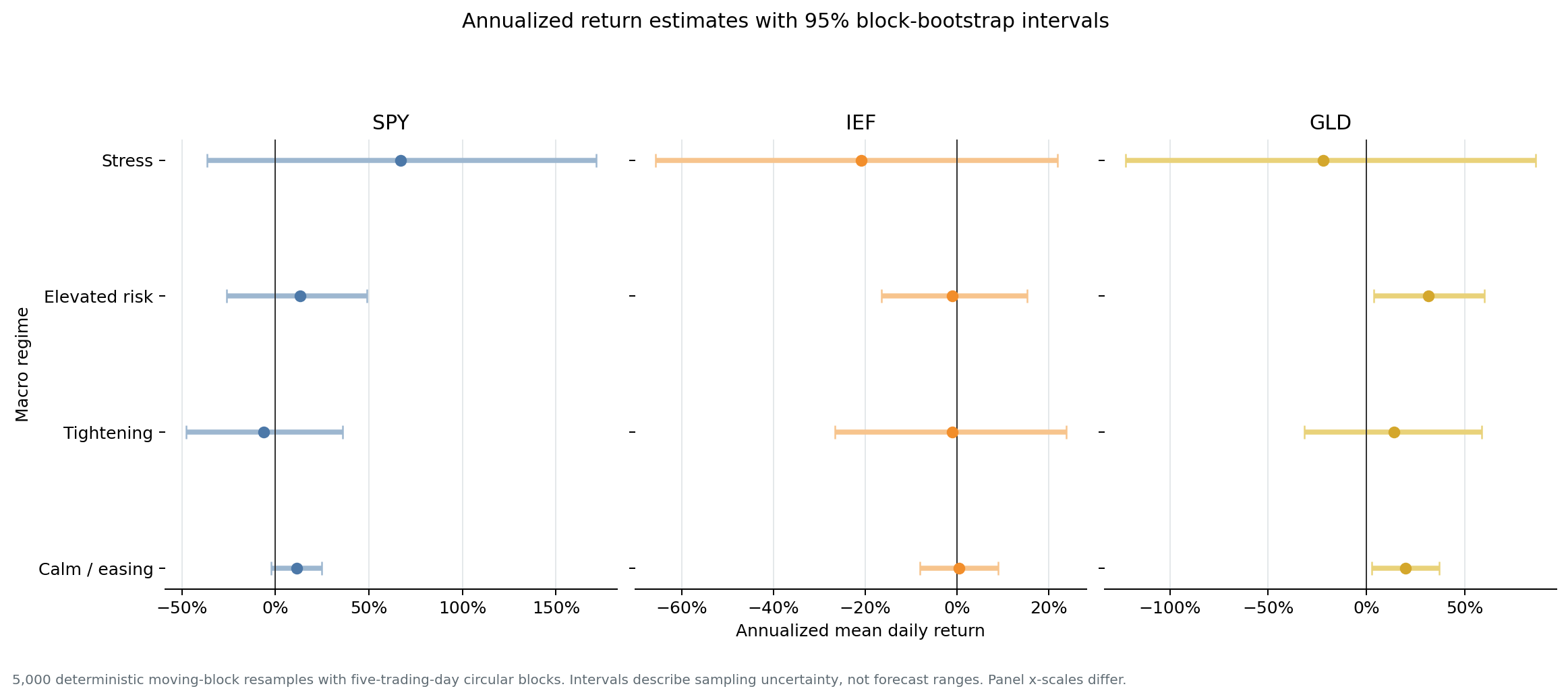
Several intervals cross zero, and Stress intervals are especially wide across assets.
The point estimate can look strong while uncertainty remains too large for a confident directional claim.
Report ranges and evidence limits. Treat the analysis as descriptive, not predictive.
Source: original project dashboard and figures. Intervals use 5,000 deterministic moving-block resamples and are not forecast ranges.
Related concepts
Method
Trust
Metrics
The regime uses information available at the previous close. This prevents the current return from using a same-day closing signal.
View implementation on GitHub ↗
result["dgs10_change_63d_pp"] = (
    result["dgs10"] - result["dgs10"].shift(YIELD_LOOKBACK_DAYS)
)
result["signal_vix"] = result["vix"].shift(1)
result["signal_dgs10"] = result["dgs10"].shift(1)
result["signal_dgs10_change_63d_pp"] = (
    result["dgs10_change_63d_pp"].shift(1)
)